You Might Also Like
Learn Coding Visually
Learn to code with interactive, live-preview playgrounds — HTML, CSS, JavaScript, React & more.
 HTML Playground42 lessons · Click-based · Live preview
 CSS PlaygroundLearn CSS with a live editor
 JavaScript Playground60 lessons · DOM · Async · Canvas
 React PlaygroundLearn React with a live code editor
 GSAP PlaygroundLearn GSAP animation interactively
 SVG Playground44 lessons · shapes · paths · animation
 SCSS Playground45 lessons · Sass modules · tokens
 Tailwind PlaygroundLearn Tailwind CSS with a live editor
 Bootstrap 5 Playground50 lessons · live preview
Canvas Gravity Particle Orbits — Free N-Body Simulation Snippet
Canvas Gravity Particle Orbits · Animations · Plain HTML, CSS & JS · Live preview
What's included
Features
About this UI Snippet
Canvas Gravity Particle Orbits — Inverse-Square Attraction From Scratch
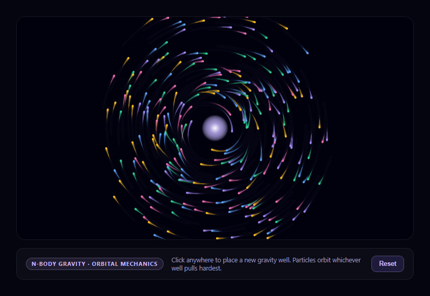
This snippet simulates hundreds of particles under real gravitational attraction toward one or more user-placed mass points, using the same inverse-square force law that governs actual orbital mechanics — implemented directly against the Canvas 2D API with no physics engine.
Newton's law of gravitation, applied per particle per well
Every frame, step() computes, for each particle and each gravity well, a force magnitude of (G * mass) / distance^2 directed along the vector between them — literally Newton's inverse-square law, just with a G constant tuned for this canvas's scale rather than real-world units. When multiple wells exist, their forces on a given particle are summed before being applied, so particles genuinely respond to the combined pull of every well simultaneously, not just the nearest one.
Softened gravity prevents infinite-force blowups
A raw inverse-square force approaches infinity as distance approaches zero, which would fling any particle that strays too close to a well out at absurd, simulation-breaking speed. step() adds a small constant (400) to the squared distance before dividing, a standard N-body simulation technique called *force softening* — it caps the maximum force at close range while leaving the force essentially unchanged at normal distances, keeping the simulation numerically stable without a special-case collision check.
Approximate initial orbital velocity, not a solved orbit
When particles are seeded, each is given a velocity roughly perpendicular to its radius vector from the central well, scaled using the standard circular-orbit-speed formula sqrt(G * mass / distance) — but randomized rather than exact. That's deliberate: an exact circular orbit would be visually static and repetitive, while the randomized approximation produces a genuine mix of elliptical orbits, slow spirals, and the occasional slingshot escape, which is far more visually interesting and still grounded in real orbital-speed math.
A second well changes everything, non-destructively
Clicking anywhere adds a new gravity well (capped at 5 total, oldest dropped first) with a randomized mass. Because the force-summing loop in step() already iterates over every well for every particle, adding a well requires no other code changes — existing particles immediately begin responding to the new combined field, visibly reorganizing their orbits or slingshotting between multiple wells.
Compare with canvas boids flocking simulation for a different from-scratch canvas simulation built on local rules instead of a global force field.
Build with AI
Build, Understand, Optimize, and Extend It With AI
Paste this snippet's HTML, CSS, and JS into an AI coding assistant like Claude and ask it to explain why the inverse-square force law needs "softening" (the small constant added to squared distance) to stay numerically stable near a gravity well, and how summing forces from multiple wells per particle is enough to make the whole simulation respond correctly to newly added wells with no other code changes. It's a great snippet to extend with an assistant — ask for two wells that themselves orbit each other (true two-body dynamics) while particles orbit both, particle-particle gravity (full N-body, at a performance cost), or a "slingshot trail" visualization that highlights particles whose speed crosses a threshold near closest approach.
Prompt to recreate it
Copy this into your AI assistant of choice to build the effect from scratch, or as a jumping-off point for your own variant:
Build an interactive "gravity particle orbit" simulation in plain HTML, CSS, and JavaScript using only the Canvas 2D API and a hand-rolled inverse-square gravity calculation — no physics engine.

Requirements:
- A canvas seeded with several hundred small particles orbiting a single central "gravity well" point, each particle given an initial velocity roughly perpendicular to its radius vector from the well, scaled using the real circular-orbit-speed formula (square root of G times well-mass divided by distance) but randomized around that value so orbits vary between tight spirals, loose ellipses, and occasional escapes rather than all being identical circles.
- Every simulation frame, for every particle, sum the gravitational force contributed by every active well using Newton's inverse-square law: force magnitude = (G * well mass) / (squared distance + a small softening constant), directed along the vector from the particle to the well. The softening constant is required — without it, a particle passing very close to a well would experience near-infinite force and be flung out at an unrealistic speed; adding a small constant to the squared distance before dividing caps the force at close range.
- Integrate that summed force into each particle's velocity and position every frame (simple explicit Euler integration is fine), and render each particle with a short fading trail (its last ~14 positions) plus a small dot at its current position.
- Let the user click anywhere on the canvas to place a new gravity well with a randomized mass there, capped at a maximum number of simultaneous wells (e.g. 5, dropping the oldest when the cap is exceeded) — existing particles should immediately begin responding to the new well's pull alongside any existing wells, since the force calculation already sums over all active wells.
- Render each gravity well as a glowing radial-gradient circle. Recycle any particle that drifts far enough off-canvas back to a random position near the center with zero velocity, rather than letting escaped particles accumulate or the particle count shrink.
- Include a Reset button that restores a single central well and re-seeds all particles, and scale for devicePixelRatio so rendering stays crisp on high-DPI screens.
Want to tighten it up first? Run this prompt through the AI Prompt Studio to score it across 8 quality dimensions, catch anti-patterns, and tune the wording for Claude, ChatGPT, or Gemini before you paste it in.
Step by step
How to Use
- 1Paste HTML, CSS, and JS260 particles orbit a central gravity well immediately.
- 2Click anywhere on the canvasA new gravity well is placed there with a randomized mass.
- 3Watch orbits reorganizeParticles respond to the combined pull of every active well.
- 4Add up to 5 wellsOlder wells are dropped once the cap is reached.
- 5Watch close passesParticles near a well curve sharply without ever flinging to infinity.
- 6Click ResetRestores a single central well and re-seeds all particles.
Real-world uses
Common Use Cases
Got questions?
Frequently Asked Questions
Yes — the force each well applies to each particle is computed as G times the well's mass divided by the squared distance between them, which is Newton's law of universal gravitation. The G constant is tuned for this canvas's arbitrary scale rather than real-world SI units, but the underlying inverse-square relationship is the genuine physics formula, not an approximation or a fake visual effect.
Because the force calculation adds a small constant (400) to the squared distance before dividing, a technique called force softening. Without it, distance approaching zero would make the force approach infinity, launching that particle at an unrealistic and simulation-breaking speed; the softening constant caps the maximum force at close range while barely affecting the force at normal simulation distances.
Every particle's acceleration each frame is the SUM of the forces from every active well, not just the nearest one. Since that summing loop already exists for a single well, adding a new one requires no special-case code — every particle immediately starts factoring the new well's pull into its combined acceleration, which is what causes visible orbit reshaping, slingshots, and captures between multiple wells.
Not exactly — initial velocities are computed using the real circular-orbit-speed formula (square root of G times mass divided by distance) but deliberately randomized around that value rather than set precisely. That randomization intentionally produces a varied mix of elliptical orbits, slow inward or outward spirals, and occasional escapes, which reads as far more dynamic and interesting than a set of perfectly repeating circular orbits would.
step() checks each particle's position against a margin outside the canvas bounds; once a particle crosses that margin, it's immediately reset to a random position near the center with zero velocity and an empty trail, effectively recycling it back into the simulation instead of letting the total particle count silently shrink over time.